Alaska Precipitation Regression
Supervised regression without a machine-learning library. Bell-shaped radial basis functions replace monomials to fit data locally rather than globally, and the coefficients come from an LU-based least-squares pipeline written by hand — first fitting a curve in 1D, then a precipitation surface over Alaska.
- Stack
- JuliaLinear AlgebraMachine LearningRegressionJupyter
- Highlights
- Radial basis functions fit locally where monomials diverge at the tails
- LU least-squares pipeline written from scratch, forward and backward substitution included
- Basis count traded off against a well-conditioned regressor matrix
The problem
Alaska has far more terrain than it has weather stations. Precipitation is measured at scattered points, but the quantity you actually want is the value everywhere in between — a smooth surface fitted to a sparse, noisy scatter of readings.
Approach
Monomials first, to show why they fail. Fitting powers of x to a noisy one-dimensional signal captures the rough shape but misses the crests, and the two curves diverge as soon as you look past the edges of the data. Every monomial is global: each one is pulled on by every measurement at once, and powers of x blow up as x grows.
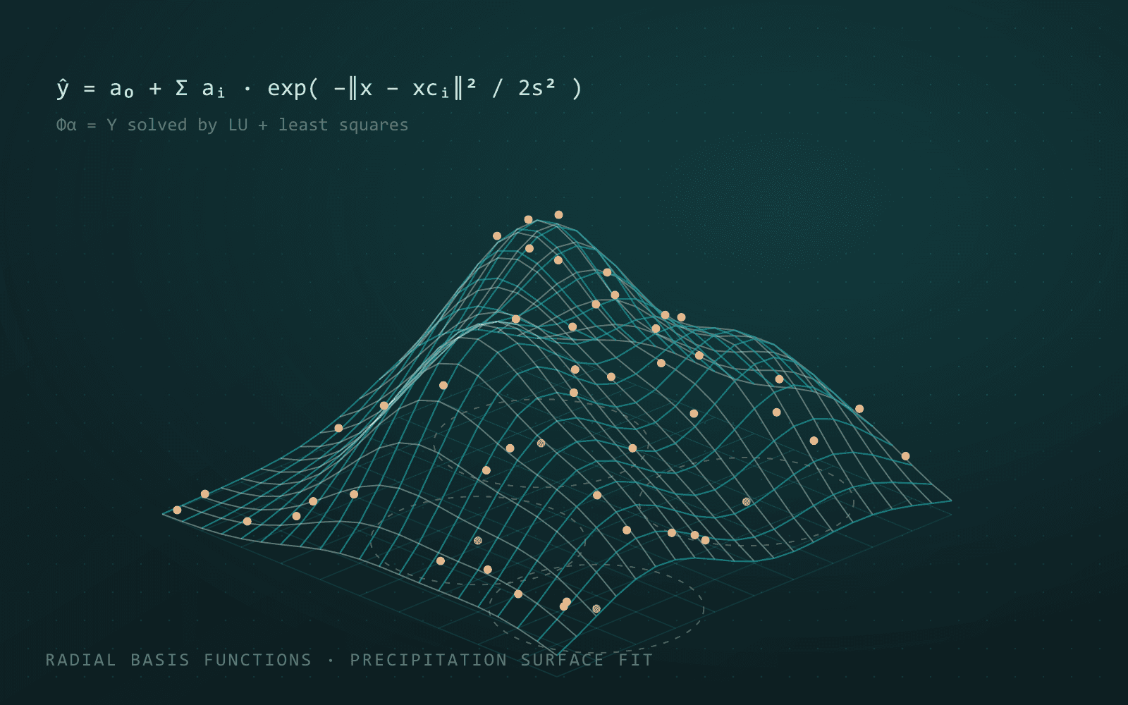
Radial basis functions instead. An RBF is a bell curve centred at a point, with a width parameter setting how far its influence reaches. Because it decays to nearly zero away from its centre, each basis element fits one local stretch of the data instead of all of it. The model is still a linear combination of nonlinear functions, so finding the coefficients is still a least-squares problem — the locality is free.
Least squares by hand. No solver shortcuts. The regressor matrix is assembled row by row, one row per measurement, and the overdetermined system is solved through an LU factorisation with permutations followed by forward and backward substitution. The result is the coefficient vector minimising the squared norm of the residual.
From a curve to a surface. The 2D case is the same algebra with wider vectors: each centre is a location on the map rather than a single x value, and the distance in the RBF exponent becomes the distance between two vectors. The regressor matrix and the LU pipeline carry over unchanged, and what comes out is a precipitation surface over Alaska.
Choosing how many bases. The number of RBFs is the real design knob. Too few and the surface underfits; too many and the centres crowd together, the columns of the regressor matrix stop being linearly independent, and the factorisation collapses into near-zero pivots. Picking it is a trade between fitting error and a system that can actually be solved.